The Software · Chapter 8.a
How does a loop become jumps?
Transcript
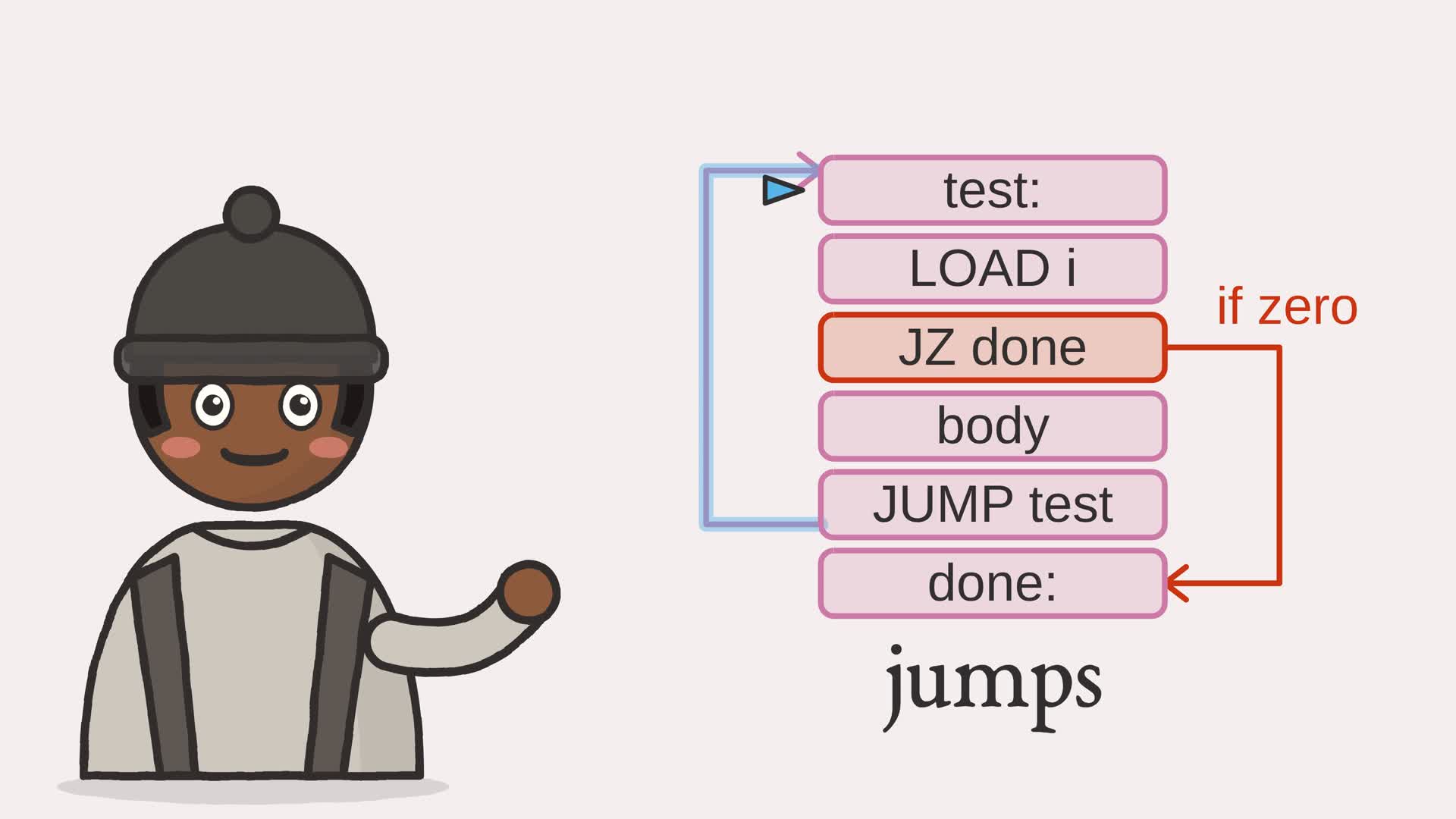
How does a loop become jumps? A processor has no loops. Just a counter and jumps.
I figured you'd copy the body out once per pass: seven passes, seven copies. But the number of passes isn't known until the program runs.
So use two jumps instead. Put a label at the top: test. Load i. If it's zero, jump past the body, to done. Otherwise, run the body. Then jump back to test, no matter what. Each pass, the counter runs down through the body, then jumps back up to test. When i hits zero, the conditional jump takes it out. Two jumps, one that asks and one that doesn't, make a loop.
So a loop is just a jump back up to the test! Compiling a loop changes how it runs, not what it means.
Set A and B below, then watch the loop compile into jumps, run, and print the product.
- The browser
- The network
- Software and languages
- The CPU
- Memory
- Arithmetic
- Logic gates
- The switch
Chapter 8 ran the imperative language by walking its tree: to execute a loop, it simply looped in Python. Chapter 7 showed that an expression need not be walked at all; it can be compiled, translated once into instructions the processor runs directly. This chapter compiles statements, and the new thing is control flow. A processor has no idea what a loop is. It has a program counter and the jumps that move it. So a while loop has to become jumps.
The instructions are Chapter 5’s: LOAD, STORE, ADD, JZ, JUMP, HALT. To keep the focus on control flow, the compiled code names its variables and labels instead of giving them numeric addresses, the form assembly takes before the linker of Chapter 6.a places it. The code generated for the loop below exceeds the sixteen words the toy machine could address. The target is an idealised version of that processor: here LOAD may also carry a literal value, memory is named and unbounded, and arithmetic does not wrap at eight bits. The compiler shown lowers only addition and a loop whose condition is a value tested against zero; a comparison such as i < b would need more cases than these.
8.a.1 A source program that counts down
The previous program counted up and compared i < b. To use only a zero test, we change it to start i at b and count down instead:
product = 0;
i = b;
while i do
  product = product + a;
  i = i + minusone;
end
The input environment is a = 6, b = 7, and minusone = -1. The grammar has no negative literals, so the negative value is supplied as an input under a name the parser accepts. This countdown computes a × b for a nonnegative integer b; a negative counter would keep moving away from zero. In ftb.codegen, this text is MULTIPLY_SOURCE, and Chapter 8’s parse turns it into the MULTIPLY tree used by both runners.
8.a.2 A loop is a test and two jumps
The shape is the one Chapter 8 drew when it traced its loop; here the compiler must emit it. Put a label at the top, the test. Evaluate the loop’s condition. If it is zero, jump past the body to the end. Otherwise run the body, then jump unconditionally back to the test. Two jumps, one conditional and one not, turn a straight line of instructions into a loop. Figure 8.a.2 shows the translation.
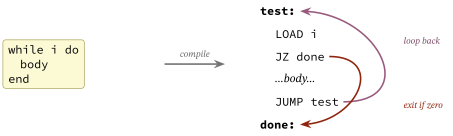
JZ exits when the test is zero; the body runs;
JUMP loops back to the test. The two jumps are the
loop.8.a.3 Expressions supply the values
Before emitting a statement, the compiler must leave its expression’s value in the accumulator. A number or variable needs one LOAD. An addition needs both sides, but the accumulator holds only one value at a time. The emitter saves the left side in a temporary, computes the right side, then adds the saved value.
Example 8.a-1. Compiling an expression into the accumulator
def _compile_expr(node, code: list, depth: int) -> None:
    """Emit instructions that leave the value of an expression in the accumulator."""
    if isinstance(node, Num):
        code.append(Instr("LOAD", node.value))          # a literal
    elif isinstance(node, Var):
        code.append(Instr("LOAD", node.name))           # from memory
    elif isinstance(node, Add):
        temp = f"_t{depth}"
        _compile_expr(node.left, code, depth + 1)
        code.append(Instr("STORE", temp))               # set the left side aside
        _compile_expr(node.right, code, depth + 1)
        code.append(Instr("ADD", temp))                 # acc = right + left
    else:
        raise ValueError(f"cannot compile expression: {node}")
At the outer addition, depth is zero and the temporary is _t0. A nested addition uses the next depth so that it cannot overwrite a value its parent still needs. Separate statements can reuse these cells. Underscores distinguish compiler temporaries from names admitted by the source grammar. With expression values available, the statement emitter can store an assignment result or test a loop condition.
Example 8.a-2. Compiling a statement
def _compile_statement(statement, code: list, counter: list) -> None:
    """Compile one statement, appending its instructions to `code`."""
    if isinstance(statement, Assign):
        _compile_expr(statement.value, code, 0)
        code.append(Instr("STORE", statement.name))
    elif isinstance(statement, While):
        number = counter[0]
        counter[0] += 1
        test, done = f"test{number}", f"done{number}"
        code.append(Instr("LABEL", test))1
        _compile_expr(statement.cond, code, 0)
        code.append(Instr("JZ", done))                  # exit when the test is zero2
        for inner in statement.body:
            _compile_statement(inner, code, counter)
        code.append(Instr("JUMP", test))                # otherwise loop back3
        code.append(Instr("LABEL", done))
    else:
        raise ValueError(f"cannot compile statement: {statement}")
- the test label, the point the loop returns to and re-checks its condition each time around
- the conditional jump out: when the condition compiles to zero, skip the body and leave the loop
- the unconditional jump back, placed after the body, which is what makes it repeat
8.a.4 Running the jumps
The machine that runs the compiled code is shaped like the processor of Chapter 5: one accumulator, one program counter. The jumps are nothing but assignments to that counter: JUMP sets it to a label, JZ sets it only when the accumulator is zero.
Example 8.a-3. The jump-driven machine
def execute(code: list, env: dict, *, max_steps: int = 10_000) -> dict:
    """Run on the idealized named-memory machine within an instruction budget.

    Raise RuntimeError on exhaustion; no partial result is returned. Labels
    count as steps, while the final HALT needs no additional step.
    """
    if type(max_steps) is not int or max_steps <= 0:
        raise ValueError("max_steps must be a positive integer")
    labels = {ins.arg: i for i, ins in enumerate(code) if ins.op == "LABEL"}
    memory = dict(env)
    accumulator = 0
    pointer = 0
    steps = 0
    while code[pointer].op != "HALT":
        if steps >= max_steps:
            raise RuntimeError(f"execution limit reached ({max_steps} steps)")
        steps += 1
        op, arg = code[pointer]
        if op == "LABEL":
            pointer += 1
        elif op == "LOAD":
            accumulator = arg if isinstance(arg, int) else memory[arg]
            pointer += 1
        elif op == "STORE":
            memory[arg] = accumulator
            pointer += 1
        elif op == "ADD":
            accumulator = accumulator + memory[arg]
            pointer += 1
        elif op == "JZ":
            pointer = labels[arg] if accumulator == 0 else pointer + 11
        elif op == "JUMP":2
            pointer = labels[arg]
        else:
            raise ValueError(f"unknown instruction {op!r}")
    return memory
- JZ: move the program counter to the label only if the accumulator is zero, otherwise fall through
- JUMP: move the counter to the label unconditionally
Like the interpreter, this runner has a finite execution budget. It raises an execution-limit error after 10,000 instructions by default, counting labels as steps. A source assignment can become several instructions, so the two runners need not exhaust their budgets together. We compare their results only when both finish.
In the instruction model, a loop is a cycle in the graph of where control can go. Figure 8.a.3 draws it.
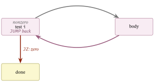
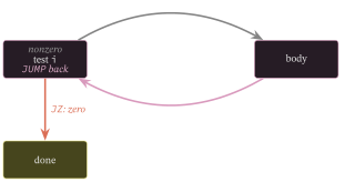
JZ sends control
to done. The loop is the cycle between test and body.8.a.5 The compiler, run
Running ftb.codegen compiles a multiplication loop, the same kind Chapter 8 interpreted, prints the jumps it became, and runs it.
the loop, compiled to jumps:
        LOAD 0
        STORE product
        LOAD b
        STORE i
test0:
        LOAD i
        JZ done0
        LOAD product
        STORE _t0
        LOAD a
        ADD _t0
        STORE product
        LOAD i
        STORE _t0
        LOAD minusone
        ADD _t0
        STORE i
        JUMP test0
done0:
        HALT

running the compiled code: product = 42
interpreting the tree:     product = 42
the two agree: True  (6 times 7 = 42)
The loop that read while i is now test0, a LOAD and a JZ done0, the body, and a JUMP test0. Running those instructions counts i down and sums a into product exactly as the interpreter did, reaching 42. The last line is the check for this example: the compiled jumps and the walked tree compute the same answer. Compiling a loop changes how it runs, not what it means.
The next chapter returns to the byte-addressed CPU and its assembled programs, then gives several programs turns on that one processor.
Exercises
- Compile an expression that adds three variables. How many temporaries does the compiler use?
- Add an if-statement to the compiler. Which labels and jumps does it need?